
Lock-Free List
Getting Familiar & Setting Up
Every once in a while, you run into a seemingly simple problem, that turns about to be much more interesting, and you open up to a whole new world.
I would like to share with you such an experience, and the subject of lock-free data structures. And it would be wise to open with a description of the issue I faced, together with its constraints to use as a segue to the topic of lock-free lists.
Introduction
While coding a certain feature in the infrastructure of the appdome engine, I realized I’m going to need to store certain data per thread.
A quick google search revealed that GCC supports the __thread keyword which specified that the variable is to be stored in each thread’s context. However, upon further examination, the implementation of this feature is quite involved in the aspect of runtime, using malloc(3) to put the data in the heap, and store the pointer in the top of the thread’s stack (in the TLS=Thread-Local-Storage).
Another option is to use the aforementioned TLS. Accessing the TLS is possible using the pthread_setspecific(3) and pthread_getspecific(3) API:
void *pthread_getspecific(pthread_key_t key);
int pthread_setspecific(pthread_key_t key, const void *value);
This way, a pointer sized data item can be stored in the TLS, and accessed using a pthread_key handle. Such a handle is obtained via the pthread_key_create(3) API:
int pthread_key_create(pthread_key_t *key, void (*destructor)(void*));
Which enables assigning a destructor function to the key. This way, arbitrary local storage can be assigned by mmap-ing and storing the pointer, and then munmap-ing in the destructor.
There is of course another way, and that is to use a lock-free hash-table.
And as there is no easy way to describe how lock-free hash-tables work, I will follow the progression of linked-lists, then lock-free linked-lists, and then lock-free hash-tables. This will also give me the opportunity of exploring what lock-free means and derive some of the properties of such algorithms and data-structures.
Linked Lists 101
In their simplest form, linked lists are usually formed of nodes which are chained together. Each node is a tuple of some data, and a pointer to the next node in the chain:
struct list_node {
    /* data item 1 */
    /*     ...     */
    /* data item n */
    struct list_node *next;
};
There is of course the extension of linked lists which have an additional pointer in each node which points to the previous node in the list. We will not, however, discuss them in this writeup, as you will soon see that dealing with a single pointer is hard enough.
Before continuing, I want to slightly modify the definition of list_node to make it purer. This will allow implementing generic functions that manipulate lists, that don’t have to rely on the actual structure of the data in the node:
struct list_node {
    struct list_node *next;
};
This way, suppose the data in the list item is:
struct list_item {
    int key;
    int value;
};
We can make it a member of a linked list by embedding the list_node structure directly into it:
struct list_item {
    int key;
    int value;
    struct list_node item_list;
};
We can even make the list item a member of several lists:
struct list_item {
    int key;
    int value;
    struct list_node item_list;
    struct list_node global_list;
};
Insert
Inserting a new list node after an existing one, requires two steps:
- Link the new node to the node following the existing one
- Link the existing node to the new node
void insert(struct list_node *node, struct list_node *new)
{
    new->next = node->next;
    node->next = new;
}
Delete
Removing a node from the list:
- Find the preceding node in the list
- Link the preceding node to the following (skip the deleted node)
void remove(struct list_node *head, struct list_node *node)
{
    struct list_node *prev = find_prev(head, node);
    prev->next = node->next;
}
Concurrency
One thing to notice about the implementation above, is that both functions are not atomic.
To demonstrate the effects of concurrency, and later measure the effectiveness of solutions, I want to write a simple emulator that would allow me to study the mechanics of concurrency without all the complexity surrounding real processors.
Emulation
To do that I will have to first define the architecture: memory (i.e. shared-state), local-state and CPU instructions.
The implementation of the emulator will be in Python as it seems the most convenient.
Memory
As we will be working with linked lists only, I will use a dictionary for the memory.
The contents of a cell can be the name of another cell, or the special name nil.
This allows me to not deal with addressing at all, but use memory cell names. For example, the following memory represents a linked list with three nodes, with the last node being the terminal node (links to nil):
dict(x='y', y='z', z='nil')
Local-state
To keep things simple, the local state will be entirely stored in “registers” (as opposed to a stack).
So each CPU will be assigned an arbitrary amount of registers labeled 0, 1 and so on.
In addition each CPU will have a special pc register the is just an index of the current instruction that is executed.
The state will also be a Python dictionary, and we can use it to set the initial state of a CPU, and we can think of the registers as function parameters.
CPU
Each CPU instruction will modify the global-state (memory) and local-state (registers) of a CPU, and in (optionally) advance the pc of the CPU.
We will start with the most basic instructions: load and store
load dst, src: Load the value of the memory pointed to by registersrcinto the registerdstclass Load: def __init__(self, dst, src): self.dst = dst self.src = src def execute(self, memory, registers): registers[self.dst] = memory[registers[self.src]] registers['pc'] += 1store src, dst: Store the value in registersrcinto the memory pointed to by the registerdstclass Store: def __init__(self, src, dst): self.src = src self.dst = dst def execute(self, memory, registers): memory[registers[self.dst]] = registers[self.src] registers['pc'] += 1
A program will simply consist of a list of instruction objects.
NOTE: The complete code of the emulator and the tests will be available in this github repository.
List Insert
We can now implement a list insert operation on our emulator.
Insert takes two parameters: the node after which to insert (first parameter - register 0), and the new node (second parameter - register 1). So the program for insert will be:
insert = [
    Load(2, 0),     # Read the contents (next) of the "after" node
    Store(2, 1),    # Set the new node to point to the next
    Store(1, 0)     # Set the "after" node to point to "new"
]
We can now test this. Our initial memory state is:
memory = {
    'x': 'y',
    'y': 'nil',
    'a': 'nil',
}
And the initial CPU state for insert(x, a) is:
registers = {
    0: 'x',
    1: 'a',
    'pc': 0,
}
Let’s run:
>>> memory
{'x': 'y', 'y': 'nil', 'a': 'nil'}
>>> _  = [op.execute(memory, registers) for op in insert]
>>> memory
{'x': 'a', 'y': 'nil', 'a': 'y'}
As you can see, node x points to a and a to y, forming the chain x > a > y.
Now let’s take this one step further. I want to be able to run two insert operations in parallel and examine the results.
But since we are dealing with 3 opcodes per insert, there is more than one way in which both instruction streams can interleave. To be more precise, there are 20 such interleave patterns (this is actually the value of the binomial coefficient C(3+3, 3)).
We can generate all the interleave patterns using these handy functions:
def interleave(*args):
    if all(len(x) == 0 for x in args):
        yield []
    for x in args:
        if len(x) == 0:
            continue
        y = x.pop(0)
        for z in interleave(*args):
            yield [y] + z
        x.insert(0, y)

def cpu_patterns(n_cpus, n_ops):
    return interleave(*([i] * n_ops for i in range(n_cpus)))
Let’s check:
>>> list(cpu_patterns(n_cpus=2, n_ops=3))
[[0, 0, 0, 1, 1, 1], [0, 0, 1, 0, 1, 1], ..., [1, 1, 1, 0, 0, 0]]
>>> len(_)
20
Looks like my math is solid.
I will now introduce the CPU class to make the code a bit prettier:
class CPU:
    def __init__(self, code, *registers):
        self.code = code
        self.regs = dict(enumerate(registers))
        self.regs['pc'] = 0
    def step(self, mem):
        opcode = self.code[self.regs['pc']]
        opcode.execute(mem, self.regs)
Now we can simulate all parallel interactions and examine the results:
for execution_order in cpu_patterns(n_cpus=2, n_ops=len(insert)):
    memory = {'x': 'y', 'y': 'nil', 'a': 'nil', 'b': 'nil'}
    cpus = [
        CPU(insert, 'x', 'a'), # insert(x, a)
        CPU(insert, 'x', 'b'), # insert(x, b)
    ]
    for cpuid in execution_order:
        cpus[cpuid].step(memory)
Here’s a visualization of all possible results:
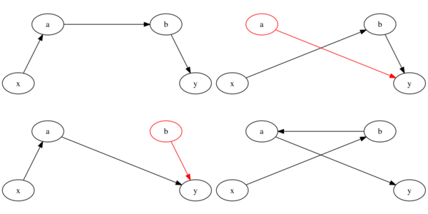
As you can see, there are 4 possible resulting states. Two of which are broken (with the broken part highlighted in red) while two are intact.
Obviously, we don’t want to end up with a broken list, but I would like to focus first on the fact that there is more than one good result.
If we want any way consistency in measuring the effectiveness of the algorithm, we need to find a way to define what is the desired result.
One possible way to do that is to attach a numerical value (a key) to each node, and then decide that the list must always be sorted according to that key.
This required expanding the memory content of a node to a struct: <pointer, key>, and together with it all the implementations of the opcodes. Python dicts are very handy:
class Store:
    def __init__(self, src, dst, key):
        self.src = src
        self.dst = dst
        self.key = key
    def execute(self, memory, registers):
        memory[registers[self.dst]][self.key] = registers[self.src]
        registers['pc'] += 1
And in addition, the insert operation must also change to first find the correct place in the list to append, and then do the list insert like before.
To do that, we will need some more opcodes:
b offset: Unconditional branch topc+offsetclass Branch: def __init__(self, offset): self.offset = offset def execute(self, memory, registers): registers['pc'] += self.offsetbg op1, op2, offset: Branch topc+offsetifop1>op2class BranchIfGreater: def __init__(self, op1, op2, offset): self.op1 = op1 self.op2 = op2 self.offset = offset def execute(self, memory, registers): if registers[self.op1] > registers[self.op2]: registers['pc'] += self.offset else: registers['pc'] += 1move dst, src: Copy the contents of registersrcto registerdstclass Move: def __init__(self, src, dst): self.src = src self.dst = dst def execute(self, memory, registers): registers[self.dst] = registers[self.src] registers['pc'] += 1
We can now implement the new insert operation:
insert_sorted = [
# RepeatSearch:
    Load(2, 0, 'next'),         # next = head->next
    Load(3, 1, 'value'),        # node->val
    Load(4, 2, 'value'),        # next->val
    BranchIfGreater(4, 3, 3),   # if node->val < next->val goto DoInsert
    Move(2, 0),                 # head = next
    Branch(-5),                 # goto RepeatSearch
# DoInsert:
    Store(2, 1, 'next'),        # node->next = next
    Store(1, 0, 'next'),        # head->next = node
]
Before actually simulating, we need to acknowledge the fact that the running times for different CPUs may vary, so one of the CPUs might get to the end of its program before the other and will have nothing to execute (which will manifest as a Python IndexError). To avoid that, we will add a halt opcode which will do nothing, not even increment pc. This way the CPU can keep executing as long as we ask it:
class Halt:
    def execute(self, memory, registers):
        pass
If we run the simulation now, we need to select some reasonable amount of cycles to interleave. I selected 14 cycles. Just to give a sense of scale, there are C(24, 12)=2,704,156 possible interlace combinations for two CPUs running 14 opcodes each. That’s a lot for poor old Python. This is probably the last time I will try to exhaust all possible combinations. After this, I will take a Monte-Carlo approach, and hope I will cover the interesting edge-cases.
Anyway, we get the following end states:
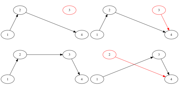 Notice that just one of them contains all the nodes AND is sorted. This is the correct end state, and we want to make it the ONLY resulting state.
Monte-Carlo
When dealing with more CPUs and more operations, we have to resort to a Monte-Carlo approach. For example, with 3 CPUs running at most 30 operations each:
for _ in range(1000000):
    memory = {
            'x': {'next': 'y', 'value': 1},
            'y': {'next': 'nil', 'value': 9},
            'a': {'next': 'nil', 'value': 2},
            'b': {'next': 'nil', 'value': 3},
            'c': {'next': 'nil', 'value': 4},
            }
    cpus = [
        CPU(insert_sorted, 'x', 'a'), # insert(x, a)
        CPU(insert_sorted, 'x', 'b'), # insert(x, b)
        CPU(insert_sorted, 'x', 'c'), # insert(x, c)
    ]
    for _ in range(30):
        random.choice(cpus).step(memory)
    aftermath.add(str(memory))
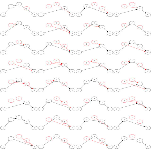 Try to spot the correct one :)
CAS to the rescue
The main problem that causes all those broken states, is that when updating the “next” field of the node after which the new node is added, we assume that it’s the same “next” that was found in the find loop. This assumption is broken in a concurrent scenario because it is not atomic.
For this purpose, the Compare-And-Set operation was invented. It is a single opcode, that read, compares and conditionally sets the contents of a memory location.
Examine the following implementation:
class CompareAndSet:
    def __init__(self, dst, key, expected, new):
        self.dst = dst
        self.expected = expected
        self.new = new
        self.key = key
    def execute(self, memory, registers):
        dst_addr = registers[self.dst]
        if memory[dst_addr][self.key] == registers[self.expected]:
            memory[dst_addr][self.key] = registers[self.new]
        registers['pc'] += 1
As you can see, this is an opportunistic operation. Meaning, the assignment might fail. We need to account for this in the code by checking if the operation succeeded, and in case of a failure to assign, we need to repeat the entire search routine and hope that the next CAS succeeds. If we think about it, we will realize that one of the CAS operations running in parallel must succeed, because if one CAS fail, that means that the contents of the memory is different, so another CPU must have succeeded.
Examine the insert operation with CAS (I took the liberty of introducing an BranchIfEqual opcode):
insert_sorted_with_cas = [
# Retry:
    Move(0, 5),
# RepeatSearch:
    Load(2, 5, 'next'),              # next = head->next
    Load(3, 1, 'value'),             # node->val
    Load(4, 2, 'value'),             # next->val
    BranchIfGreater(4, 3, 3),        # if node->val < next->val goto DoInsert
    Move(2, 5),                      # head = next
    Branch(-5),                      # goto RepeatSearch
# DoInsert:
    Store(2, 1, 'next'),             # node->next = next
    CompareAndSet(5, 'next', 2, 1),  # if (node->next == next) node->next = new
    Load(3, 5, 'next'),
    BranchIfEqual(3, 1, 2),          # if (node->next == new) goto Done
    Branch(-11),                     # goto Retry
# Done:
    Halt(),
]
Let’s see the simulation results.
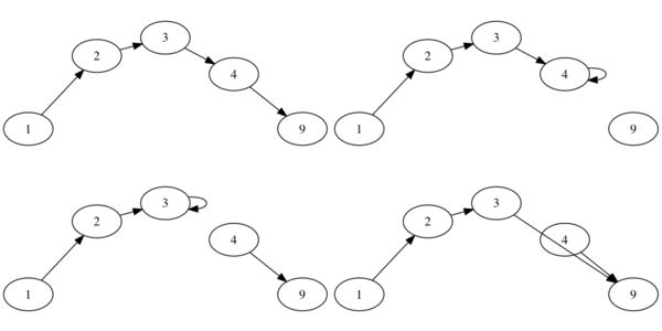
Huh?! What happened here?
Well, the sharper of you might have already realized the flaw. You see, they way we verified the CAS succeeded was by examining the content of the memory following the CAS. However, this can lead to a situation where the CAS succeeded, but since the Load operation is performed later, we may see a value written there by another CPU.
This is why CAS usually writes the success/failure status of the assignment to some register. This register can the be tested and branches can be taken.
As we are the authors of this architecture, we can expand CompareAndSwap to take an additional operand: the branch offset in case of a failure:
class CompareAndSet:
    def __init__(self, dst, key, expected, new, failure):
        self.dst = dst
        self.expected = expected
        self.new = new
        self.key = key
        self.failure = failure
    def execute(self, memory, registers):
        dst_addr = registers[self.dst]
        if memory[dst_addr][self.key] == registers[self.expected]:
            memory[dst_addr][self.key] = registers[self.new]
            registers['pc'] += 1
        else:
            registers['pc'] += self.failure
And the updated insert routine:
insert_sorted_with_cas = [
# Retry:
    Move(0, 5),
# RepeatSearch:
    Load(2, 5, 'next'),                 # next = head->next
    Load(3, 1, 'value'),                # node->val
    Load(4, 2, 'value'),                # next->val
    BranchIfGreater(4, 3, 3),           # if node->val < next->val goto DoInsert
    Move(2, 5),                         # head = next
    Branch(-5),                         # goto RepeatSearch
# DoInsert:
    Store(2, 1, 'next'),                # node->next = next
    CompareAndSet(5, 'next', 2, 1, -8), # if (node->next == next) node->next = new
                                        # else goto Retry
    Halt(),
]
Now we get just a single final state which is (not surprisingly) the correct one.
Performance
It is interesting to measure just what can be gained by this, albeit simple, algorithm in terms of parallelizing work.
To do that, we first need a way to measure the elapsed time for a simulation. By measuring time, I don’t mean the time it takes to run the simulation, but rather the amount of in-simulation cycles that passes from the first instruction, to the last.
We need to take note of two observations:
- Two (or more) opcodes ran by different CPUs can occupy the same time slot
- Two opcodes run by the same CPU can not occupy the same time slot
Also, we will start with a list of all CPUs, each round we select a random CPU from the list, execute an opcode, and then if the CPU reached the end of the program (please no comments about the halting problem) we remove it from the list. Once the list empties, we know all the insertions are done and we can take note of the elapsed cycles.
We can do this for a varying number of CPUs, each CPU will add its own node with a distinct key, and see how well the running time scales. In addition, since we are doing a Monte-Carlo simulation, we need to run each simulation several times, and then take the average and variance of the measurements.
Of course, the measurements by themselves are meaningless, and what matters in the comparison to a serial execution of all the inserts (also, averaged on several runs).
The results of a sweep from 2 to 83 (I got impatient and stopped the simulation) CPUs yielded the following running times for parallel and sequential runs:
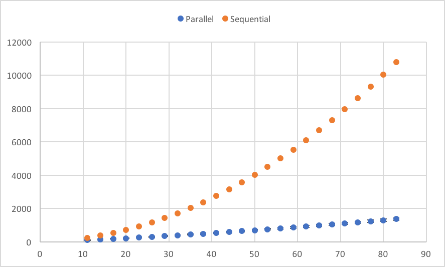
And the “improvement” of the parallel algorithm is the ratio:
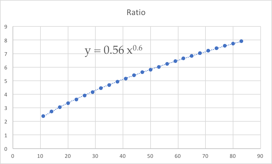
As you can see, the improvement is not linear to the number of CPU, but slightly lower, i.e. doubling the number of CPUs will increase throughput by some factor less that 2, and the more CPUs we add, the harder it will be to get an increase in performance. The optimal number of CPUs will be determined by the economics of the problem.
Summary
Well, that was a mouthful. I believe I will give it a rest for now.
There’s a lot we did not talk about yet. But we did manage to:
- Get familiar with linked lists
- Design and implement our own architecture
- Explore concurrency with sorted insert operations on a list
- Learn about CAS and how it helps attain consistency in face of concurrency
- Do some laboratory experiments and derive some interesting findings
In the next post, we will explore the remove operation on a lock-free linked list, the problems that will arise, and their solutions.
See you soon!